Swerve Drive Forwards Kinematics

This is part two of my swerve drive math writeup. Read part one which covers reverse kinematics
here

Swerve drive forwards kinematics, or calculating a robot velocity from sensor positions is a bit more complicated than the reverse kinematics covered in the earlier post.

One could assume that the robot will execute all commands perfectly; that is, if I use the reverse kinematics to command the robot to move at 10 m/s forwards, I could then assume the robot would travel 10 m/s forwards and calculate a pose through vector integration.

In reality, this is not the case. Different motor powers, gearbox efficiencies and the fact that the wheels cannot match the correct heading immediately all create deviations that add accumulate over time.

Both of the methods detailed in this article will yield a robot velocity in robot space (i.e. “robot-centric” velocity). Conversion to a “field-centric” velocity is possible (and recommended) through vector rotation. Vector integration can be used to accumulate the velocities into a displacement.

The Easy Case

If the swerve module positions are symmetric (that is, their displacements relative to the robot center of rotation sum to zero), the forwards kinematics can be simplified greatly.

(Math details) Wait, isn't this the only case?

It is worth noting that the center of rotation is arbitrary; any swerve drive movement can be expressed as a combination of rotation and translation around any center of rotation. Furthermore, any module layout will have a "geometric center," relative to which the module displacements will sum to zero. That said, it can be useful to have a consistent center of rotation between forwards and reverse kinematics, that in some cases may not be the geometric center of the modules.

This case covers almost every competition robot I have seen; most teams use square or rectangular drive base configuration.

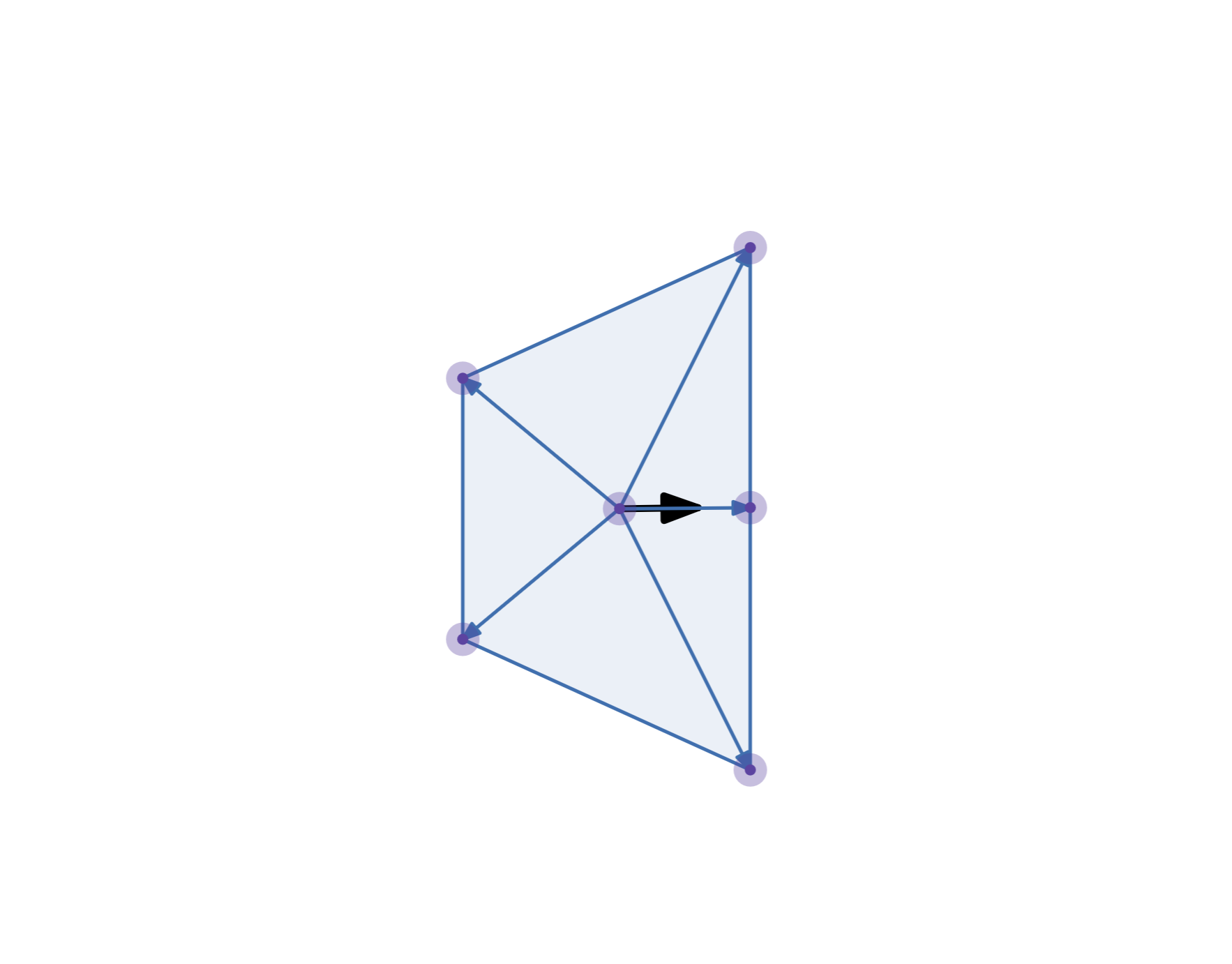
To start, one can find the robot’s translational velocity by taking the average of the module velocities. Because the module positions sum to zero, any torques that the modules exert on the robot will cancel out.

• v_R is the robot velocity
• v_m is a module velocity

\[v_R = \frac{\sum \vec{v}_m}{(Number Of Modules)}\]

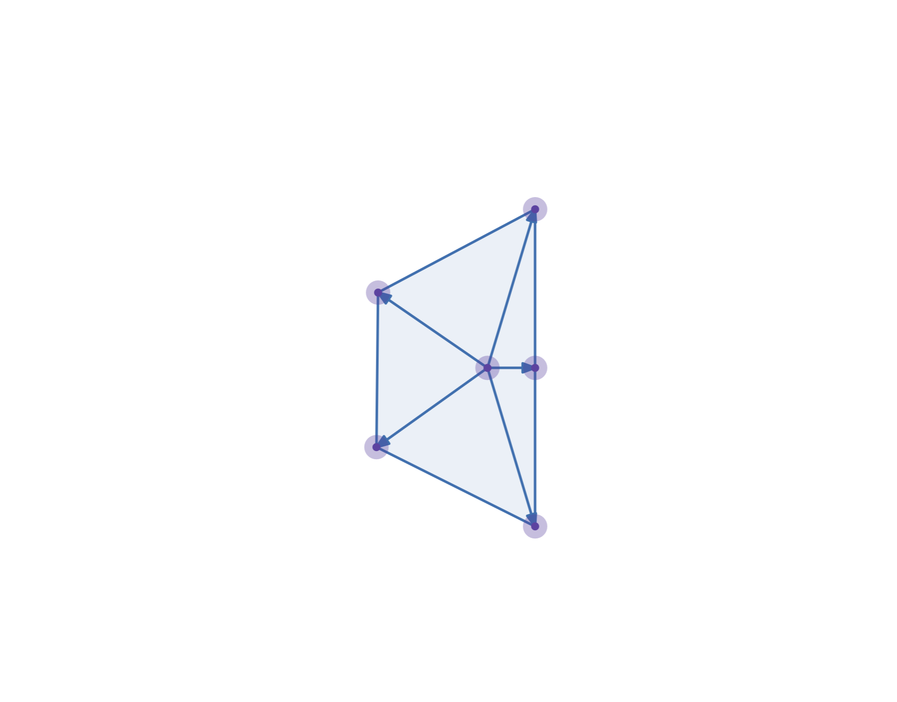
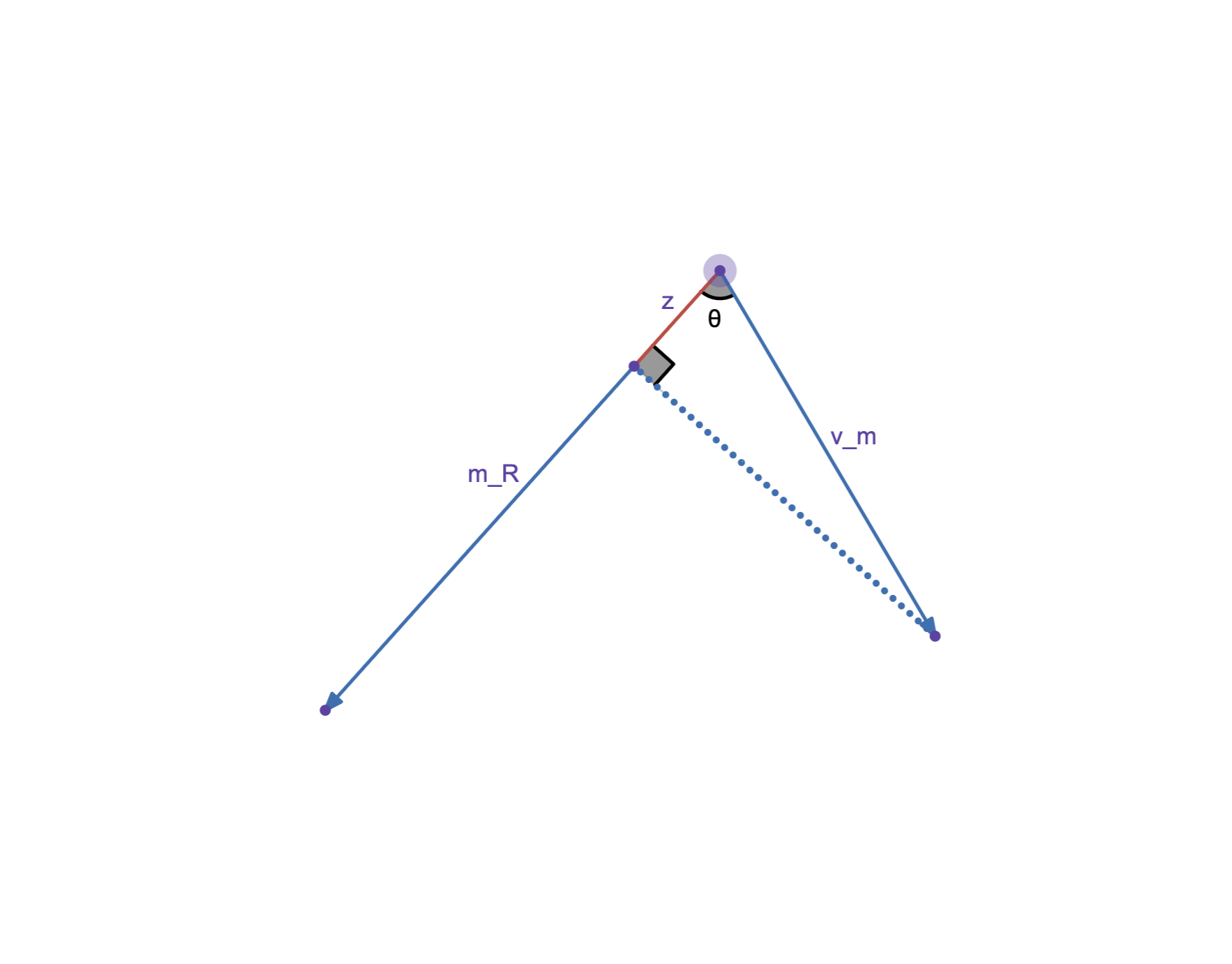
The robot’s angular velocity can be found by averaging the components of the module velocities that are perpendicular to the module’s displacement vector. (Or parallel to the module’s rotation vector that was already calculated for use in reverse kinematics.)

• a_R is the robot angular speed
• m_r is a module rotation vector
• v_m is a module velocity

\[a_R = \frac{\sum{\frac{\vec{v}_m \cdot \vec{m}_r}{|\vec{m}_r|}}}{(Number Of Modules)}\]

Math Shortcut Explanation

Consider the above image. The length z is the component of the module velocity (v_m) that is perpendicular to the module rotation vector. We know that $$ cos(\theta) = \frac{z}{|\vec{v}_m|} $$ Therefore $$ |\vec{v}_m| \cdot cos(\theta) = z $$ We also know that $$ cos(\theta) = \frac{\vec{v}_m \cdot \vec{m}_r}{|\vec{v}_m| \cdot |\vec{m}_r|} $$ Substitution yields $$ z = \frac{\vec{v}_m \cdot \vec{m}_r}{|\vec{v}_m| \cdot |\vec{m}_r|} \cdot |\vec{v}_m| $$ Which simplifies to $$ z = \frac{\vec{v}_m \cdot \vec{m}_r}{|\vec{m}_r|} $$

The universal case

This method for calculating forwards odometry relies on the fact that each module’s velocity is a combination of a robot translational and angular velocity, and that the robot is a rigid body; the angular and translational velocities of all modules are the same.

Expressed as an equation, given any two modules:

\[\left\{ \begin{array}{ll} \vec{v}_{m1} = \vec{v}_R + a_R \cdot \vec{m}_1r \\ \vec{v}_{m2} = \vec{v}_R + a_R \cdot \vec{m}_2r \end{array} \right.\]

The module velocities, v_m and the module rotation vectors m_r are both known. Solving this system of equations yields the translation and rotation of the robot.

In Quail’s implementation of this algorithm, I wrote a function that generates a list of all the possible module pairs and averages the robot velocities after solving on each pair.